 (logit),
 In working with binomial data, one is interested in modeling
the probability of occurrence of an event of interest as a function of one or
more covariates. The most commonly used regression model for such data is the
logistic regression model in which the log odds, (logit),
is modeled as a linear function of the covariates. As shown in Specification of More General Models, the default GMBO/PECAN model corresponds to logistic regression. Because of the generality of the models available in EPICURE, it is straightforward to use GMBO/PECAN to fit generalized models for the odds. However, in some cases it is useful to model functions other than the logit or log odds. The function describing the relationship between the binomial probability and the regression function is called the link. In addition to the default odds/logit link, it is also possible to use GMBO/PECAN to fit models that involve complementary log and identity links. The complementary log link is

which includes the complementary log-log link
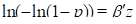
as a special (default) case. The identity link is

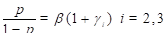
In this section we will present examples illustrating the use of alternative link functions. These data were used by Wacholder (Wacholder 1986) to illustrate the use of alternatives to logistic regression. For our purposes, we will focus on the effect of alcohol consumption and ignore the smoking and socioeconomic status information in the data. The models to be fit are equivalent to

where  index three levels of alcohol
consumption. The first example involves a complementary log-log link, the second
an identity link, and the third a log link.
index three levels of alcohol
consumption. The first example involves a complementary log-log link, the second
an identity link, and the third a log link.
Example 5.7 Modeling the Odds: Changing the Default Subterm
The data are read and the alcohol, smoking, and socioeconomic variables are created with the following commands:
NAMES x n @
INPUT ../exdata/sholom.dat @
TRAN alcohol = 4 - GL(3,1) ; socio = GL(3,6) ; smoker = GL(2,3) @
LEVELS alcohol socio smoker @
CASES x
N n
The function GL(n,r) produces a variable with n distinct values, 1 to n. Each value is repeated r times. The whole sequence is repeated as many times as necessary. Thus, the command GL(2,3) leads to a variable whose first 8 values are 1,1,2,2,3,3,1,1. This results in a set of integer-coded variables that can be used as factors in the subsequent analyses.
In this example we will fit models of the form

that is, we will model the odds directly. It is not necessary to change the link function to do this. Rather, one simply uses the linear subterm of term 0 instead of the default log-linear subterm. This is easily done using the LINEAR 0 model specification command. It is also necessary to remove the default intercept from the log-linear subterm of term 0. Finally, it is necessary to provide a valid initial value for the intercept or any other parameter that directly estimates an odds. This is necessary because the default initial value (0.00) is not included inside the parameter space for such parameters. For these models, initial values must be positive.
The commands to specify and fit a simple model for the odds in this population are
LINEAR 0 %CON:1 @
FIT -%CON @
The first command specifies the model of interest and provides an acceptable starting value (1). The FIT command is used not only to fit the model but also to remove the default intercept from the log-linear subterm of term 0. An alternative command sequence with the same effect is
FITOPT LINEAR 0 @
LOGLINEAR 0 - %CON @
FIT %CON:1 @
In this command sequence, the FITOPT command is used to change the default subterm, that is, the term updated by model formulae given on a FIT command to be the linear subterm of term 0. The LOGLINEAR command is used to remove the default intercept. Finally, the model is specified and fit using the FIT command with an appropriate model formula. The parameter summary table produced by either set of commands is shown below.
Output 5.6 A direct model for the odds
Binomial odds regression
Additive excess relative risk T0 * (1 + T1 + T2 + ...)
x is used for cases
n is used for number of trials
Parameter Summary Table
# Name Estimate Std.Err. Test Stat. P value
-- ---------------------------- ---------- --------- ---------- --------
Linear term 0
1 %CON..................... 0.1222 0.01308 9.345 < 0.001
Records used 18
Deviance 33.2051
AIC 35.2051
Pearson Chi2 37.182 Degrees of freedom 17
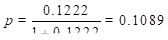
We see that the odds is estimated to be 0.1222 with a standard error of 0.0131. This estimate corresponds to
Assuming we have changed the default subterm as indicated above, the commands
FIT + alcohol @
FIT -%CON @
fit a model with direct estimates of the odds for each alcohol category. The output below shows the results for the first model.
Output 5.7 An odds difference model
FIT + alcohol @
Iter Step Deviance
0 0 33.2051
1 0 23.9900
2 0 23.9635
3 0 23.9635
Binomial odds regression
Additive excess relative risk T0 * (1 + T1 + T2 + ...)
x is used for cases
n is used for number of trials
Parameter Summary Table
# Name Estimate Std.Err. Test Stat. P value
-- ---------------------------- ---------- --------- ---------- --------
Linear term 0
1 %CON..................... 0.09881 0.01465 6.746 < 0.001
3 alcohol_2................ 0.01230 0.03274 0.3756 > 0.5
4 alcohol_3................ 0.1117 0.04349 2.569 0.0102
Records used 18
Deviance 23.9635
AIC 29.9635
Pearson Chi2 23.8906 Degrees of freedom 15
Note that the effect of alcohol consumption at level 1 is not shown because this parameter is aliased. The intercept (%CON) is the maximum likelihood estimate for the odds in the first alcohol consumption category. The other two parameters in the model are the difference in group 1 and groups 2 and 3 odds, respectively. Thus, the odds for group 2 is estimated as 0.09881+0.01230=0.11111, while the estimated odds for group 3 is 0.21051. These estimates are obtained directly from the next model, in which the intercept is dropped.
Example 5.8 Using Generalized Models: Estimates of Odds Ratios
In this example we fit a model equivalent to the last model in the previous example; however, we consider an alternative parameterization in which we estimate one minus the odds ratios for alcohol consumption in groups 2 and 3 relative to group 1. The model to be fit can be written
In this model  is the odds for group 1
and
is the odds for group 1
and  are the odds ratios. This model
involves two subterms in two terms. The intercept parameter, , is included in the linear subterm of
term 0, while the odds ratio parameters are in the linear subterm of term
1.
are the odds ratios. This model
involves two subterms in two terms. The intercept parameter, , is included in the linear subterm of
term 0, while the odds ratio parameters are in the linear subterm of term
1.
The commands to specify and fit this model are
LINEAR 1 alcohol @
LINEAR 0 %CON:0.1 @
PARAMETER 2=0 @
FIT @
The first two commands are standard EPICURE model specification commands. Note that we specified an explicit initial value for the %CON parameter. The PARAMETER command is used to fix the parameter associated with alcohol group 1 to be 0. Since one of the parameters in the full model is aliased and since the intrinsic aliasing checks in EPICURE do not extend across terms or subterms, we use the PARAMETER command to explicitly fix the parameter associated with alcohol group 1 at 0. The program would fit the model and note that one parameter is aliased even if this were not done. However, interpretation of the parameters would not be straightforward. The output for this model is shown below.
Output 5.8 An odds ratio model
Binomial odds regression
Additive excess relative risk T0 * (1 + T1 + T2 + ...)
x is used for cases
n is used for number of trials
Parameter Summary Table
# Name Estimate Std.Err. Test Stat. P value
-- ---------------------------- ---------- --------- ---------- --------
Linear term 0
1 %CON..................... 0.09881 0.01465 6.746 < 0.001
Linear term 1
2 alcohol_1................ 0.000 Aliased
3 alcohol_2................ 0.1244 0.34 0.366 > 0.5
4 alcohol_3................ 1.131 0.521 2.17 0.03
Records used 18
Deviance 23.9635
AIC 29.9635
Pearson Chi2 23.8906 Degrees of freedom 15
The odds ratios for groups 2 and 3 are 1.12 and 2.13, respectively.
Example 5.9 Changing the Link: Complementary Log-Log Models
In this example we will fit the same models as in the last example, but we will make use of the complementary log link. With this link the regression model is

Because the default subterm is the log-linear subterm of term 0, the default model, that is, the model specified by model formulae given with the FIT command, is a complementary log-log model:

To work with the complementary log link, we must first change the link. This is done with the command
LINK COMP @
In addition to changing the link function, this command removes any parameters from the current model, sets the default subterm to be the log-linear subterm of term 0, and turns on the automatic intercept option. Thus, if the next command is a FIT command with no arguments, we fit the simplest complementary log-log model:

The estimate of  in this model is
-2.160, which is easily seen to be equivalent to the value obtained in Example 5.7 in
which the odds was estimated to be 0.1222.
in this model is
-2.160, which is easily seen to be equivalent to the value obtained in Example 5.7 in
which the odds was estimated to be 0.1222.
We can fit alternative models that include alcohol effects with the commands
FIT alcohol @
FIT -%CON @
As in the examples in the last section, the alcohol parameters in the former model estimate contrasts (differences on the complementary log-log scale) between alcohol consumption groups 2 and 3 and consumption group 1. Dropping the intercept, as in the latter example, does not change the fit but leads to a different parameterization in which the parameter estimates correspond to the complementary log-log values for the three groups. The model summary table for this model is shown below.
Output 5.9 A complementary log-log model
Binomial regression with complementary log link
Additive excess relative risk T0 * (1 + T1 + T2 + ...)
x is used for cases
n is used for number of trials
Parameter Summary Table
# Name Estimate Std.Err. Test Stat. P value
-- ---------------------------- ---------- --------- ---------- --------
Log-linear term 0
1 alcohol_1................ -2.362 0.1415 -16.7 < 0.001
2 alcohol_2................ -2.250 0.2501 -8.997 < 0.001
3 alcohol_3................ -1.655 0.177 -9.349 < 0.001
Records used 18
Deviance 23.9635
AIC 29.9635
Pearson Chi2 23.8906 Degrees of freedom 15
As you can see from this figure, the model summary table
includes information on the current link and indicates the interpretation of the
default model. (This description is correct only for models that contain no
parameters in other subterms.) Note that the deviance is identical to that
obtained for the equivalent odds models shown in Output 5.7 and
Output 5.8. This
equivalence holds because we are working with simple main-effects models. It is
easy to compute the probabilities associated with three levels of alcohol
consumption. For example, the probability for consumption group 1 is 0.08993
 . The probabilities for the other two
groups are 0.10003 and 0.17394, respectively.
. The probabilities for the other two
groups are 0.10003 and 0.17394, respectively.
Example 5.10 Using the Identity Link
In this example we fit the same models as in the last two examples using the identity link. With this link the regression model is

Because the default subterm is the linear subterm of term 0,
the default model is one in which the probabilities of interest are modeled as a
linear function of the parameters. As was the case with the odds models
considered earlier, there are implicit constraints on the parameter space
because  must be between 0 and 1. Thus,
maximum likelihood estimates may not exist for models of this type, which
include continuous covariates. Also, as was the case for the odds models, the
default initial parameter value (0) is not appropriate for main effects.
must be between 0 and 1. Thus,
maximum likelihood estimates may not exist for models of this type, which
include continuous covariates. Also, as was the case for the odds models, the
default initial parameter value (0) is not appropriate for main effects.
The LINK ID command is used to choose the identity link. In addition to changing the link function, this command removes any parameters from the current model, sets the default subterm to be the linear subterm of term 0, and turns on the automatic intercept option. The intercept is included in the linear subterm of term 0.
LINK ID @
The command
FIT %CON:0.1 @
can be used to obtain the maximum likelihood estimate of the
disease probability in this sample. The explicit initialization is necessary in
this example because the default initial value of 0 leads to estimates that are
not in the allowable range, and the maximization stops with an error in this
case. The estimated case probability is 0.1089 with a standard error of 0.01038.
These estimates are simply 
and 
where  is the number of cases and
  the total number of subjects in
the study. In this example is 98 and is 900.
the total number of subjects in
the study. In this example is 98 and is 900.
We can fit models that include alcohol effects with the commands
FIT alcohol @
FIT alcohol:0.1 - %CON @
In the first model, the intercept is the estimated probability of being a case in alcohol group 1, while the other two parameters are the differences between the probabilities in the other two groups and group 1. The fit summary table for this model is shown below.
Output 5.10 A probability difference model
Binomial regression with identity link
Additive excess relative risk T0 * (1 + T1 + T2 + ...)
x is used for cases
n is used for number of trials
Parameter Summary Table
# Name Estimate Std.Err. Test Stat. P value
-- ---------------------------- ---------- --------- ---------- --------
Linear term 0
1 %CON..................... 0.08993 0.01213 7.412 < 0.001
3 alcohol_2................ 0.01007 0.02664 0.3781 > 0.5
4 alcohol_3................ 0.08398 0.03046 2.757 0.00583
Records used 18
Deviance 23.9635
AIC 29.9635
Pearson Chi2 23.8906 Degrees of freedom 15
We see from this table that the group 2 probability is 0.010 greater than that in group 1, while the group 3 probability is 0.084 greater than that in group 1. The standard errors suggest that there is a significant difference in the case probabilities for groups 1 and 3. However, one should be wary of using Wald tests in nonstandard models such as this one. Likelihood ratio tests or likelihood-based bounds provide a more reliable guide to the statistical significance in these models. Using the commands
BOUNDS 3 @
BOUNDS 4 @
we obtain 95 percent likelihood bounds of (-0.038; 0.067) and (0.028; 0.15) for the two contrasts. The following series of commands can be used to obtain the likelihood ratio test of the hypothesis of no difference in the case probability for groups 1 and 3:
NULL @
PARAMETER 4=0 2=0 @
FIT @
LRT
The first command is used to indicate that the current (full) model is to be used as the comparison model in the test. The PARAMETER command is used to force the contrast for group 3 (parameter 4) to be 0. It is also necessary to fix parameter 2 at 0 to keep the program from fitting an alternative form of the current model. The PARAMETER command must be used here since alcohol is a categorical variable and we are only constraining some of the levels. The FIT command fits the constrained model, and the LRT command computes the likelihood ratio statistic. The output from this command indicates that the statistic is -9.080 with -1 degrees of freedom and a P-value of 0.0026. The statistic is negative because we used the full model as a base model in the comparison.