
The examples in this section illustrate features of risk modeling for cohort studies with AMFIT. The data on the cohort have been grouped into four dose categories with no additional stratification. The data set contains a record for each dose category. These four records are:
|
1 |
6 |
2500 |
0 |
|
2 |
4 |
1000 |
10 |
|
3 |
8 |
1000 |
20 |
|
4 |
6 |
350 |
25 |
The first column contains a category index variable, while the second and third columns contain the number of cases and the total number of person-years accumulated during the course of the study. We will call these variables dcat, cases, and pyr, respectively. The mean dose (dose) received by people in each category is in the fourth column. The data are read from a file called MOCK.DAT. Although the material is presented in a series of examples, it is assumed that the commands are given in a single session in the order in which they are discussed here. Also, the emphasis in this section concerns model specification and fitting. Issues related to hypothesis testing will be touched upon in the examples in the next section.
Example 7.1 Point and Interval Estimates for a Crude Rate
The data set can be described and read with the following commands:
NAMES dcat cases pyr dose @
INPUT ../exdata/mock.dat @
We begin with a simple model of the form
in which the parameter β is the log of the crude rate observed in this study. Two key variables are required to fit a model in AMFIT, a case-count variable and a person-years variable. It is not necessary to specify these variables explicitly in this example because they can be determined by the program from the variable names cases and pyr. Since the key variables are known, the simple model described above can be specified and fit using the command
FIT @
The output produced by this command is shown below.
Output 7.1 Simple AMFIT model
Iter Step Deviance
0 0 9409.394
1 0 3343.289
2 0 1141.555
3 0 360.640
4 0 100.351
5 0 26.7878
6 0 13.1502
7 0 12.2176
8 0 12.2104
9 0 12.2104
Piece-wise exponential regression
Additive excess relative risk T0 * (1 + T1 + T2 + ...)
cases is used for cases
pyr is used for person years
Parameter Summary Table
# Name Estimate Std.Err. Test Stat. P value
-- ---------------------------- ---------- --------- ---------- --------
Log-linear term 0
1 %CON..................... -5.309 0.2041 -26.01 < 0.001
Records used 4
Deviance 12.2104
AIC 14.2104
Pearson Chi2 15.8624 Degrees of freedom 3
The output begins with a summary of the progress of the fitting algorithm. For each iteration, the program prints the deviance. For AMFIT models the deviance is minus twice the difference between the log likelihood for the fitted model and that which would be obtained in a fully saturated model, that is, a model with a parameter for each cell in the event-time table. (Technical Details contains formulae for the deviance values printed by AMFIT and the other EPICURE programs.) The iteration summary also includes information on step halving (discussed in Technical Details). Step halving refers to a modification to the default step that occurs whenever the standard step fails to increase the log likelihood (decrease the deviance).
As illustrated here, the AMFIT fit summary table begins with a
header indicating that this is a piecewise exponential regression model (in this
example there is only one piece). This is followed by a description of the form
of the fitted model, which is a product additive excess model in this case.
(Model forms available in AMFIT were described in Fitting Models with
Epicure) This general information is followed by a
summary of the current key variables. Although not illustrated here, a
description of the active subset is written when a selection is in effect. The
parameter estimate table is printed following the model and selection summary
information. This table has one line for each parameter in the model (in this
case there is only a single parameter). The information for each parameter
includes a) the parameter number, which is needed for some commands, and the
name of the covariate associated with the parameter; b) the parameter estimate;
c) its asymptotic standard error; d) test statistic for estimated parameters or
the score test for fixed (non-aliased) parameters; and e) the P-value for the
hypothesis of the test statistic. The last few lines of an AMFIT fit
summary table contain the number of records used, deviance, its degrees of
freedom, the AIC statistic, and the Pearson  statistic. As will become
clearer in later examples, the parameter summary table is divided into sections
labeled by the subterm type and term number. In this example the parameter is in
the loglinear subterm of term 0. This is the default subterm for AMFIT models.
statistic. As will become
clearer in later examples, the parameter summary table is divided into sections
labeled by the subterm type and term number. In this example the parameter is in
the loglinear subterm of term 0. This is the default subterm for AMFIT models.
In this example the parameter estimate is -5.309 with an estimated standard error of 0.2041. The crude rate, which is easier to interpret, is computed as e-5.309=0.0049 cases per person-year. This rate is included as part of the table of Wald bounds produced by the command
CI @
The Wald bound table for this model is shown in Output 7.2.
Output
7.2 Wald bound table for a crude rate parameter
CI @
95% Confidence Bounds
# Name Estimate Std. Err. Lower Upper
-- ---------------------------- ---------- --------- -------- --------
Log-linear term 0
1 %CON..................... -5.309 0.2041 -5.709 -4.909
EXP(estimate) 0.004948 1.226 0.003317 0.007383
This table contains the parameter estimate, standard error, and 95 percent bounds for each parameter in the model. (Options can be used to change the confidence level.) As illustrated here, the estimate, the standard error, and the bounds are exponentiated for parameters in loglinear subterms. In this case, as in many others, the exponentiated estimate and bounds are of direct interest. Fitting Models with EPICURE contains a discussion of confidence bound computation options.
Example 7.2 Category-Specific Relative and Absolute Risk Estimates
We will now fit various models that provide risk estimates for each of the four dose categories. These models illustrate the use of categorical variables as covariates in a fit. The first step is to indicate that dcat is a categorical variable. This can be done with the command
LEVELS dcat @
which produces the following output:
DCAT has 4 levels from 1 to 4
indicating that dcat has four levels that are coded with the values 1, 2, 3, and 4.
Once this has been done we use the command
FIT dcat @
to fit a model that provides estimates for the risk in each dose category. The fit summary table for this example is shown in Output 7.3.
Output 7.3 Parameter estimates for a categorical dose response model: relative risks
Piece-wise exponential regression
Additive excess relative risk T0 * (1 + T1 + T2 + ...)
cases is used for cases
pyr is used for person years
Parameter Summary Table
# Name Estimate Std.Err. Test Stat. P value
-- ---------------------------- ---------- --------- ---------- --------
Log-linear term 0
1 %CON..................... -6.032 0.4082 -14.78 < 0.001
3 dcat_2................... 0.5108 0.6455 0.7914 0.429
4 dcat_3................... 1.204 0.5401 2.229 0.0258
5 dcat_4................... 1.966 0.5774 3.405 < 0.001
Records used 4
Deviance 0
AIC 8
Pearson Chi2 2.41571e-19 Degrees of freedom 0
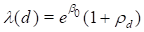
Since this model has one parameter for each record in the input data set, it fits the data perfectly, a situation that would not normally arise in more realistic examples. Although the model specification did not contain an intercept, the fitted model does. This is because by default in AMFIT (and GMBO) an intercept is always included in the loglinear subterm of term 0. We will show how to remove the intercept later in this example. The current model can be written
where d is the dose category index. As written this model contains five parameters, but because there are only four dose categories, one of these parameters is aliased. AMFIT detects this type of aliasing before fitting the model and automatically removes from the model the parameter corresponding to the first dose category. Thus, the parameter summary table does not include an entry for parameter 2, the log relative risk for the first dose category.
The intercept in this model is the log rate for the first dose
category, while the  parameters are the log relative
risks for the dose categories. As in the last example, we can use the CI command to obtain Wald bounds and background rate and
relative risk parameters. The point estimate of the background (category 1) rate
is 0.0024, while the category-specific relative risk estimates are 1.67, 3.33,
and 7.14.
parameters are the log relative
risks for the dose categories. As in the last example, we can use the CI command to obtain Wald bounds and background rate and
relative risk parameters. The point estimate of the background (category 1) rate
is 0.0024, while the category-specific relative risk estimates are 1.67, 3.33,
and 7.14.
If the intercept is dropped from this model, we obtain an equivalent model of the form

in which the parameters correspond to the absolute risk in each category. This model is specified and fit with the command
FIT -%CON @
The leading  in this command
indicates that %CON is to be dropped from the model.
Dropping the default intercept turns off the option, which forces automatic
inclusion of the intercept. Automatic inclusion of the intercept can be turned
back on by explicitly adding %CON to the loglinear
subterm of term 0 or with the FITOPT INTERCEPT
command. The parameter summary table for the new model is shown in Output
7.4.
in this command
indicates that %CON is to be dropped from the model.
Dropping the default intercept turns off the option, which forces automatic
inclusion of the intercept. Automatic inclusion of the intercept can be turned
back on by explicitly adding %CON to the loglinear
subterm of term 0 or with the FITOPT INTERCEPT
command. The parameter summary table for the new model is shown in Output
7.4.
Output 7.4 Parameter estimates for a categorical dose response model: absolute risks
Parameter Summary Table
# Name Estimate Std.Err. Test Stat. P value
-- ---------------------------- ---------- --------- ---------- --------
Log-linear term 0
1 dcat_1................... -6.032 0.4082 -14.78 < 0.001
2 dcat_2................... -5.521 0.5 -11.04 < 0.001
3 dcat_3................... -4.828 0.3536 -13.66 < 0.001
4 dcat_4................... -4.066 0.4082 -9.96 < 0.001
Records used 4
Deviance 0
AIC 8
Pearson Chi2 9.66283e-19 Degrees of freedom 0
Since this model is simply an alternative parameterization of the first model in this example, the deviance is the same as before. Using the CI command or a calculator, we can see that the point estimates of the category-specific absolute risks are, not surprisingly, 0.0024, 0.004, 0.008, and 0.01714.
Example 7.3 An Exponential Relative Risk Model
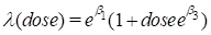
In this example we use the dose covariate to fit a simple dose response model. The model is a simple relative risk model that is written as

In some contexts this model might be called an exponential or multiplicative relative risk model. The command to specify and fit this model is
FIT %CON dose @
The inclusion of %CON is necessary because it was dropped in the previous model, which suppressed the automatic inclusion of an intercept. Output 7.5 presents the parameter summary table for this model. This output indicates that a one-unit change in dose is associated with a 7 percent change in the relative risk.
Output 7.5 Parameter estimates for a multiplicative relative risk model
Parameter Summary Table
# Name Estimate Std.Err. Test Stat. P value
-- ---------------------------- ---------- --------- ---------- --------
Log-linear term 0
1 %CON..................... -6.133 0.3823 -16.04 < 0.001
2 dose..................... 0.07303 0.02217 3.294 < 0.001
Records used 4
Deviance 0.644865
AIC 4.64486
Pearson Chi2 0.662483 Degrees of freedom 2
Example 7.4 Using Alternative Models: Modeling the Excess Relative Risk
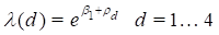
In this example we will specify and fit a model of the form

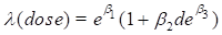
We will also consider a parameterization of the form
In both models, the relative risk is described as a linear function of dose. Such models are sometimes called additive relative risk models. In the first of these models, the parameter β2 describes the change in the excess relative risk (that is, one minus the relative risk) per unit dose, while in the second, β3 is the logarithm of this change. As long as β2 is positive, these two models are equivalent. But if β2 is negative, it is not possible to estimate β3 in the second model. Although these are nonstandard models, both are included in EPICURE’s default class of product additive excess models as described in Equation 4.8.
All of the models considered thus far in this chapter could be specified and fit using only the FIT command. Because of the nature of the excess relative risk models considered here, we must make use of the LINEAR and LOGLINEAR subterm specification commands.
To start afresh, we will begin with the command
NOMODEL
which clears the current parametric model and restores automatic intercept inclusion. (Although not relevant here, this command does not affect stratification.)
Two commands are necessary to specify and fit the first model. These commands are
LINEAR 1 dose @
FIT @
The first command indicates that dose is to be included in the linear subterm of term 1. The FIT command causes the model to be fit. It is not necessary to indicate %CON because it is included in the loglinear subterm of term 0 by default. The parameter summary table produced by these commands is shown in Output 7.6.
Output 7.6 Parameter estimates for an excess relative risk model
Parameter Summary Table
# Name Estimate Std.Err. Test Stat. P value
-- ---------------------------- ---------- --------- ---------- --------
Log-linear term 0
1 %CON..................... -6.108 0.4166 -14.66 < 0.001
Linear term 1
2 dose..................... 0.1532 0.1011 1.516 0.13
Records used 4
Deviance 1.8127
AIC 5.8127
Pearson Chi2 1.96058 Degrees of freedom 2
This parameter summary table differs from those seen thus far in that it includes two sections. The first section describes the parameters in the loglinear subterm of term 0, while the second section provides information on the parameters in the linear subterm of term 1. The estimate for parameter 2 indicates that the relative risk changes by 0.15 per unit change in dose.
We now fit the alternative parameterization described above. To specify this model, it is useful to think of the model as of the form
in which  is set equal to and
fixed at 1. With this in mind, it should be easy to see that the following
commands will specify and fit the desired model:
is set equal to and
fixed at 1. With this in mind, it should be easy to see that the following
commands will specify and fit the desired model:
LINEAR 1 dose=1 @
LOGLINEAR 1 %CON @
FIT @
The inclusion of dose in the linear subterm of term 1 with its associated parameter set equal to 1 is indicated by the use of the parameter initialization operator (=) following the covariate name. The parameter to be estimated is indicated by the inclusion of %CON in the loglinear subterm of term 1. The parameter summary table produced by these commands is shown in Output 7.7.
Output 7.7 Parameter estimates for a reparameterized excess relative risk model
Parameter Summary Table
# Name Estimate Std.Err. Test Stat. P value
-- ---------------------------- ---------- --------- ---------- --------
Log-linear term 0
1 %CON..................... -6.108 0.4166 -14.66 < 0.001
Linear term 1
2 dose..................... 1.000 Aliased
Log-linear term 1
3 %CON..................... -1.876 0.6597 -2.843 0.00447
Records used 4
Deviance 1.8127
AIC 5.8127
Pearson Chi2 1.96051 Degrees of freedom 2
This parameter summary table contains a separate section for
each subterm in the model. The dose parameter is equal to 1 but is reported as
aliased because, if it were to be estimated, it would be redundant. As expected,
the deviance is the same as in the last model, and the estimate of  is equal to the logarithm of the
dose parameter in the earlier model.
is equal to the logarithm of the
dose parameter in the earlier model.
We conclude this section by fitting a model that provides direct estimates of the dose-category-specific excess relative risks. This model can be written as
where, as before, d represents an index for the dose categories. As written, this model contains a redundant parameter, but we will specify and fit the model without doing anything special to deal with this redundancy. The commands to replace the previous model with this one are
LOGLINEAR 1 @
LINEAR 1 dcat @
FIT @
The LOGLINEAR command without a model formula removes all parameters in the associated subterm. The LINEAR command causes the dose parameter in the previous model to be replaced by the dose category indicators defined by dcat. Output 7.8 shows some of the output produced for this fit.
Output 7.8 Parameter estimates for a categorical excess relative risk model
Piece-wise exponential regression
Additive excess relative risk T0 * (1 + T1 + T2 + ...)
cases is used for cases
pyr is used for person years
Parameter Summary Table
# Name Estimate Std.Err. Test Stat. P value
-- ---------------------------- ---------- --------- ---------- --------
Log-linear term 0
1 %CON..................... -6.108 Aliased
Linear term 1
2 dcat_1................... 0.07894 0.4405 0.1792 > 0.5
3 dcat_2................... 0.7982 0.8991 0.8878 0.375
4 dcat_3................... 2.596 1.272 2.042 0.0412
5 dcat_4................... 6.707 3.146 2.132 0.033
Records used 4
Deviance 0
AIC 8
Pearson Chi2 1.31477e-31 Degrees of freedom 0
First note the parameter 1 is identified as aliased. This reflects the fact that the model includes parameters for each dose category in the excess relative risk (Linear term 1) and a parameter for the baseline rate (%CON in loglinear 0) so it is possible to estimate only four of the five parameters in the model. While EPICURE does check for intrinsic aliasing within each subterm, the program does not check for aliased parameters across subterms. However, when parameters are aliased, it will be detected as the model is fit, and the program will fix as many of the parameters as needed to allow fitting the model. In this example, the %CON term in the baseline is treated as aliased with the associated parameter fixed at its value at the time the aliasing was detected. Because of this rather arbitrary decision, it is difficult to determine the (excess relative risks) for the different dose categories.
Even though the parameter estimates for the last fit are “correct”, they would be easier to interpret if we made a more rational choice for the baseline category. In this case a more appropriate parameterization would force the excess relative risk parameter associated with the first (zero dose) category to be zero. This is easily done using the PARAMETER command. This command allows us to specify initial values and put simple constraints on specific parameters in a model. Parameters must be referenced by number in the PARAMETER command. For this example we want to force the parameter associated with the first dose category to be 0 and then refit the model. The commands to do this are
PARAMETER 2=0 @
FIT @
Note again that the = parameter initialization operator is used to initialize and fix the parameter at 0. The parameter summary table for this fit is shown in Output 7.9.
Output 7.9 Parameter estimates for a categorical excess relative risk model after introducing an explicit constraint
Parameter Summary Table
# Name Estimate Std.Err. Test Stat. P value
-- ---------------------------- ---------- --------- ---------- --------
Log-linear term 0
1 %CON..................... -6.032 0.4082 -14.78 < 0.001
Linear term 1
2 dcat_1................... 0.000 Aliased
3 dcat_2................... 0.6667 1.076 0.6197 > 0.5
4 dcat_3................... 2.333 1.8 1.296 0.195
5 dcat_4................... 6.143 4.124 1.49 0.136
Records used 4
Deviance 0
AIC 8
Pearson Chi2 9.1486e-20 Degrees of freedom 0
The parameter estimates in this model are quite easy to interpret and agree with those for the equivalent multiplicative model fit earlier.
Example 7.5 Using Alternative Models: An Absolute Excess Risk Model
In this example we show how to change the form of the model. We are interested in obtaining direct estimates of the change in the absolute excess risk associated with a unit in dose. The model to be considered here is a reparameterization of the simple excess relative model considered at the beginning of the last example. This model of interest can be written as
In this parameterization the model is not included in the default class of product excess risk models. Therefore, it is necessary to instruct the program to use the alternative class of additive risk models. This is done with the command
ADD @
Following this command, the models being fit will be additive models of the form

This command does not change the parameters (if any) in the current model, but it does change the interpretation of parameters in terms other than term 0. We can now specify and fit the model of interest with the commands
LINEAR 1 dose @
FIT @
The fit summary for this model is shown in Output 7.10.
Output 7.10 Fit summary for an additive model
Piece-wise exponential regression
Additive T0 + T1 + T2 + ...
cases is used for cases
pyr is used for person years
Parameter Summary Table
# Name Estimate Std.Err. Test Stat. P value
-- ---------------------------- ---------- --------- ---------- --------
Log-linear term 0
1 %CON..................... -6.108 0.4165 -14.66 < 0.001
Linear term 1
2 dose..................... 0.0003409 0.0001227 2.777 0.00548
Records used 4
Deviance 1.8127
AIC 5.8127
Pearson Chi2 1.96069 Degrees of freedom 2
Note that the description of the model type has changed to reflect the change made with the ADD command. From the parameter estimates we see that the absolute risk is estimated to change by 0.00034 cases per person-year for a unit change in dose.