A More Complex Example: Hazard Functions, Survival Curves, and Stratification

In this section we use the lung cancer data from Kalbfleisch and Prentice (1980, pp 60 --69) to illustrate additional features of PEANUTS, including the use of stratified models and procedures for the computation and plotting of survival curves and other functions of the hazard function. The data set includes information on the variables described in the following table.

Description of the Lung Cancer Data

Name	Description
cases	Case indicator variable (0 censored; 1 uncensored)
time	Time of death or censoring
status	Performance status (Karnofsky scale) 10-90
dxmnths	Months since diagnosis
age	Age in years at diagnosis
prior	Prior therapy (0 no; 10 yes)
trmnt	Treatment group (1 standard; 2 test)
cell	Cell type (1 squamous; 2 small cell; 3 adenocarcinoma; 0 large cell)

The data are stored in a file called LUNG.DAT. The first ten records from this file are:

In the examples in this and the following section, we consider the effect of treatment and various covariates on the survival time. The cell-type covariate is treated as a categorical variable with four levels. In this section we will continue to work with the default exponential proportional hazards model. Alternative models are considered in the next section.

Example 6.5 Reading the Data and Fitting an Unstratified Exponential Risk Model

The first few commands in this example are

! Commands to read the lung cancer trial data

NAMES cases time status dxmnths age prior trmnt cell @

INPUT ../exdata/lung.dat @

TRAN stat50 = status - 50 ; age60 = age - 60 ; trmnt = trmnt - 1 @

LEVELS cell @

The first line in this file is a comment. The first command specifies the names of the variables to be read, and the second command instructs the program to read the data file. The third command specifies transformations that define centered versions of the status and age variables and recodes trmnt and prior to be a binary(0/1) indicators. The final command indicates that cell is to be used as a categorical variable. The number of levels and origin for cell is determined by the program.

Once the data have been read, we fit the following model for the relative risk

where indexes the cell type. This model can be specified and fit with the command

FIT cell stat50 age60 dxmnths prior trmnt @

The parameter summary table for this fit is shown below.

Output 6.7 Parameter estimate table for a multivariate model

Hazard function regression

Additive excess relative risk T0 * (1 + T1 + T2 + ...)

cases is used for cases

time is used for survival time

Parameter Summary Table

# Name Estimate Std.Err. Test Stat. P value

-- ---------------------------- ---------- --------- ---------- --------

Log-linear term 0

2 cell_1................... -0.3991 0.2826 -1.412 0.158

3 cell_2................... 0.4526 0.2664 1.699 0.0893

4 cell_3................... 0.7911 0.3026 2.614 0.00895

5 stat50................... -0.03270 0.005493 -5.954 < 0.001

6 age60.................... -0.008563 0.009305 -0.9203 0.357

7 dxmnths.................. -1.724e-05 0.009115 -0.001891 > 0.5

8 prior.................... 0.07388 0.2322 0.3182 > 0.5

9 trmnt.................... -0.2861 0.207 -1.382 0.167

Records used 137

-2 * log-likelihood 950.006 Free parameters 8

AIC 966.006 Informative risk sets 97

Non-informative risk sets 1

The parameter summary table is similar to those we have seen before; however, following the deviance summary there is a message indicating that there is one non-informative risk set. A risk set is said to be non-informative if its contribution to the information matrix is zero. In this example, this occurs because the observation with the longest survival time is a failure.

We will not discuss the results in this table in detail; rather, we simply note that cell type and status (Karnofsky score) are the only variables that appear to have significant effects on survival.

Note that only three of the four cell-type parameters are shown. This is because one of these parameters is aliased with the background hazard. In this case, the program determined that one of the cell-type parameters was aliased and automatically chose to drop the first cell-type (type 0, large-cell carcinoma). Thus, the background hazard in this model describes the risk for a patient with large-cell carcinoma. As shown in the next example, we can use the SCURV command to obtain information about the background hazard and related functions.

Example 6.6 Estimating the Hazard and Plotting the Survival Curve

We will begin by plotting the survival curve, that is, the probability that a person remains alive by time t. The survival curve is determined from the hazard function, which is the instantaneous probability of failure in the small time interval conditional on survival to time t. PEANUTS estimates the baseline hazard, that is, , in the models described above, using the method developed by Breslow (1974) and described in Technical Details. The survival function and cumulative hazard function are computed from the estimated hazard function. The SCURV command requests estimation of the hazard, cumulative hazard, and survival functions and produces plots of these functions versus time or log time.

Assuming that none of the defaults have been changed, the command

SCURV @

instructs the program to compute the hazard, cumulative hazard, and survival function at each distinct failure time in the data set used for the most recently fitted model and to plot the survival function versus time. A short summary of the survival function will be written to the log file. This summary give the survival probabilities at the 90^th, 75^th, 50^th and 25^th and 10^th percentiles of the survival distribution. For this example the summary table looks like this

Relative Risk = 1

Percentile Time

90% 12.00

75% 25.00

50% 59.00

25% 117.0

10% 186.0

In the presence of heavy censored data the lower percentiles may not be estimable. In this case they will be shown as missing (.). When the TABLE option is used, a detailed table giving the number of events, the number at risk, the hazard and cumulative hazard estimates, and the estimated survival probability at each failure time is written to the log file. The break key (CTRL-C on most machines) can be used to stop the display of long tables.

The estimates are for the baseline hazard, that is, for a person with a zero covariate vector. Whether these estimates describe the survival of a person of interest depends on how the covariates in the model have been defined. In the model fit in the first example, the covariates were defined so that the baseline hazard describes a subject receiving the standard treatment (trmnt) who entered the study at the time immediately after diagnosis (dxmnths) with large-cell carcinoma (cell). The subject had no prior therapy (prior), a Karnofsky score of 50 (stat50) and was 60 years of age at diagnosis (age60).

Output 6.8 contains the first few and the last few records of the hazard function table written to the log file when the SCURV TABLE @ command is used for the model fit to the lung cancer data in the last example.

Output 6.8 Hazard function estimate table for the lung cancer data (partial)

Relative Risk = 1

Time Events At Risk Hazard Cumlative Survial

Hazard Prob.

1.000 2 137 0.01212 0.01212 0.9879

2.000 1 135 0.006162 0.01829 0.9819

3.000 1 134 0.006266 0.02455 0.9757

4.000 1 133 0.006414 0.03097 0.9695

7.000 3 132 0.01950 0.05046 0.9508

.. .. ..

553.0 1 4 0.6480 6.745 0.001176

587.0 1 3 0.9036 7.649 0.0004765

991.0 1 2 1.627 9.276 9.365e-05

999.0 1 1 4.866 14.14 7.218e-07

As can be seen in the output, the table of estimates begins with a banner labeling the columns. The first column contains the failure times, the second column lists the number of events that took place at that time, and the third column shows the number of people at risk. The last three columns contain the estimated hazard, cumulative hazard, and survivor function, respectively. It is indicated that the results in this table are for stratum number 1. In this case there are no additional strata, however, for stratified models a separate table is produced for each stratum.

The FROM and TO subcommands can be used to limit the range of times for which records are written to the log file. Using these csubommands only affects what is displayed and not the range of data that are plotted.

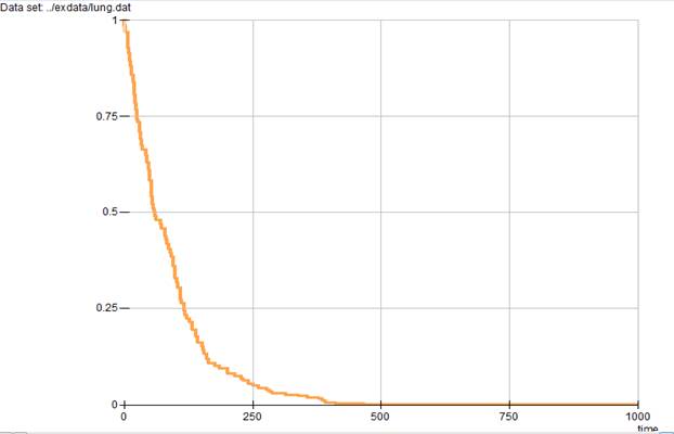
Both of the commands given above produce the survival curve plot shown in Output 6.9.

In this plot the horizontal axis describes time, while the vertical axis describes the survival probability. From this plot it appears that survival probability falls very rapidly during the first 200 days.

Output 6.9 Survival curve for the lung cancer data

The following command allows us to take a closer look at the survival curve during the period up to (about) 200 days. This is done using the TMAX subcommand as in the following example.

SCURV TMAX 200 @

The plot produced by this command is shown in Output 6.10. Although not illustrated here, the TMIN subcommand can be used to specify a minimum value for the time scale.

The plot range always includes the user-specified range.

Example 6.7 Hazard and Cumulative Hazard Function Plots

The survival curve is not the only, nor generally the most informative, plot one might want to make for these data. The command

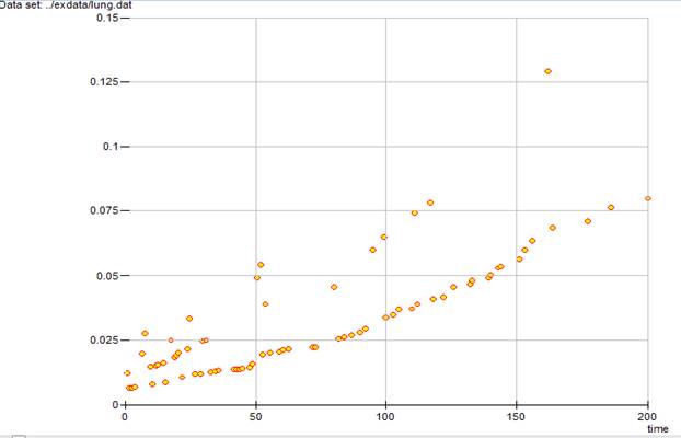
SCURV HAZA TMAX 200 @

produces the hazard function plot over the 0 to 200 day range shown in Output 6.11.

Although for these data the hazard generally increases with time, the hazard is not necessarily a monotone function of time and, unlike the survival curve, the points are not connected.

Output 6.10 Survival curve with restricted time scale for the lung cancer data

Output 6.11 Hazard function plot for the lung cancer data

The cumulative hazard function (minus the log of the survival function) can be plotted using the command

SCURV CHAZ @

The plot produced by this command is shown in Output 6.12.

Output 6.12 Cumulative hazard function for the lung cancer data

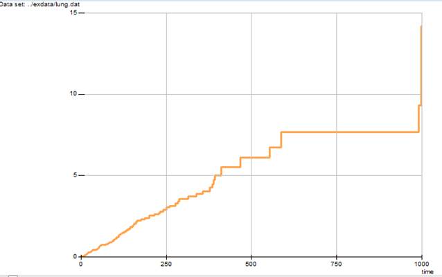
Note that the cumulative hazard function is plotted as a step function. Also note that because we did not explicitly specify the time axis restriction, the time scale reverted to the full range. Although most SCURV subcommands set options that remain in effect until changed by the user, the TMIN, TMAX, and TO specifications must be given each time they are used.

The log cumulative hazard is often more informative than is the cumulative hazard function. In PEANUTS, one can plot the logarithm of any of the survival-related quantities by adding L as a prefix on the appropriate subcommand, that is, LSURV, LHAZA, and LCHAZ for plots of the log survival, hazard, and cumulative hazard functions, respectively. (As mentioned above, the log survival function is simply minus the cumulative hazard.) The LOGTIME subcommand is used to request a log time scale in any of the survival-related function plots. Like the other plot-type subcommands, once requested the log time scale remains in effect until explicitly canceled by the user with the TIME subcommand.

The final command in this example,

SCURV LCHAZ LOGTIME TMAX 200 AS plotdata @

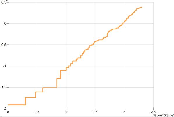
plots the log cumulative hazard against log time for times less than 200. Note that the time range restriction is given in untransformed units (that is, days in this data set) even though the plot is to be drawn using a log scale for the time axis. The resulting plot is shown in Output 6.13.

Output 6.13 A log cumulative hazard versus log time plot for the lung cancer data

The AS

Example 6.8 Changing the Baseline Model for Estimates and Plots

The REFVECTOR and REFMODIFY commands can be used in conjunction with the SCURV command to compute and plot hazard and survival functions for covariates other than the baseline hazard (that is, the hazard when all covariates in the model are equal to 0). For example, in the model fit above, the baseline hazard is the risk for a person with a large cell carcinoma (cell = 0) with a Karnofsky score of 50 diagnosed at age 60 with no prior treatment with follow-up from the date of diagnosis. If we are interested in the relative risk and survival function for a person with squamous cell carcinoma case (cell = 1) diagnosed at age 40 with a Karnofsky score of 90 diagnosed 6 months before the start of follow-up with no prior therapy, we can define a reference vector using the command:

refmodify prior = 0 ;

stat50 = 90 - 50 ;

dxmnths = 6 ;

age60 = 40 - 60;

trmnt = 1 ;

cell = 1 ;

This commands defines a vector in which the covariates in the model take on values corresponding to the conditions described above. Transformations specified using the REFMODIFY command affect only the reference vector. Once the reference vector has been defined, the SCURV command can be used to compute the hazard and survival function for this covariate vector. For SCURV @ the result is:

Reference vector covariates:

cell 1.0000 stat50 40.000 age60 -20.000

dxmnths 6.0000 prior 0.0000 trmnt 1.0000

Relative Risk = 0.16168

Percentile Time

90% 54.00

75% 143.0

50% 384.0

25% 991.0

10% .

Since a reference vector is defined, the first section of the SCURV output lists the value of the model covariates for the reference vector. This is followed by a line giving the relative risk for these covariate values and then the survival function summary. If the table option were used, the hazard function table would be shown. The plot gives the survival function at the reference vector. In this example the relative risk is a lot less than 1 so people survive considerably longer than those with the baseline covariates.

The command REFVECTOR CLEAR @ is used to clear the reference vector.

It is also possible to reparameterize and refit this model so that the fitted baseline rate corresponds to the reference vector described above. To do this we define new covariates using the following transformations:

TRAN

notrmnt = 1 - trmnt ;

stat90 = status - 90 ;

dxmn6 = dxmnths - 6 ;

age40 = age - 40 ;

We then specify the reparameterized model using the command

LOGL 0 cell stat90 age40 dxmn6 prior notrmnt @

We use LOGL 0 instead of the FIT command because we want to place an additional restriction on the parameter values prior to fitting the model. In particular, because squamous-cell carcinoma is cell-type 1 (which is parameter 2 in the model), we use the command

PARA 2=0 @

to force the parameter associated with squamous-cell cancer to be 0, which makes this the base type. Once this has been done, we fit the model with the command

FIT @

The parameter summary table for this fit is shown below.

Output 6.14 Parameter estimate table for a re-parameterized model

Hazard function regression

Additive excess relative risk T0 * (1 + T1 + T2 + ...)

cases is used for cases

time is used for survival time

Parameter Summary Table

# Name Estimate Std.Err. Test Stat. P value

-- ---------------------------- ---------- --------- ---------- --------

Log-linear term 0

1 cell_0................... 0.3991 0.2826 1.412 0.158

2 cell_1................... 0.000 Aliased

3 cell_2................... 0.8517 0.2752 3.096 0.00196

4 cell_3................... 1.190 0.3008 3.957 < 0.001

5 stat90................... -0.03270 0.005493 -5.954 < 0.001

6 age40.................... -0.008563 0.009305 -0.9203 0.357

7 dxmn6.................... -1.724e-05 0.009115 -0.001891 > 0.5

8 prior.................... 0.07388 0.2322 0.3182 > 0.5

9 notrmnt.................. 0.2861 0.207 1.382 0.167

Records used 137

-2 * log-likelihood 950.006 Free parameters 8

AIC 966.006 Informative risk sets 97

Non-informative risk sets 1

Note that the deviance is the same as before because this is simply an alternative form of the same model.

We can now print the hazard function estimate table and plot the survival curve for these data using the command

SCURV SURV TIME @

The survival function summary for this reparameterized model is

Relative Risk = 1

Percentile Time

90% 54.00

75% 143.0

50% 384.0

25% 991.0

10% .

The relative risk is given as 1 since we reparameterized the model to use a different baseline, and the survival function is the same as that seen above based on the original parameterization with a reference vector. The survival curve plot is shown in Output 6.15.

Output 6.15 Survival Curve for a re-parameterized model

Example 6.9 Smoothing the Hazard Function Estimate

It is also possible to estimate and plot a smoothed hazard funciton using the kernel smoothing method suggested in Breslow and Day (1987, pp 193 -195), which is described in Technical Details. This is done using the SMOOTH command. This command requires that you specify a bandwidth for the smoother in units that correspond to those of the time scale used for the modeling. To produce a smoothed estimate, you must specify the bandwidth to be used for the smoothing function. The bandwidth must be a non-negative number, with 0 corresponding to the usual unsmoothed estimate and any large value resulting in a smoothed estimate. When a bandwidth of is specified, the hazard function is estimated only for the interval , where and are the smallest and largest failure times in the data set or the upper and lower times indicated using the TLIMIT option of the SMOOTH command.

We illustrate this feature with the command

SMOOTH 30 TMAX 300 @

which requests a smoothed hazard function plot with a bandwidth of 30 days for the smoother. The time scale is limited to the first 300 days. In this analysis, the units for the hazard on the veritcal axis are cases per day. Unless explicitly suppressed by the user, a hazard estimate table will be printed by this command. (You can use the break key, usually CTRL-C, to stop the printing of an unwanted hazard estimate table.)

The output from this command is shown in Output 6.16.

Output 6.16 A smoothed hazard function plot

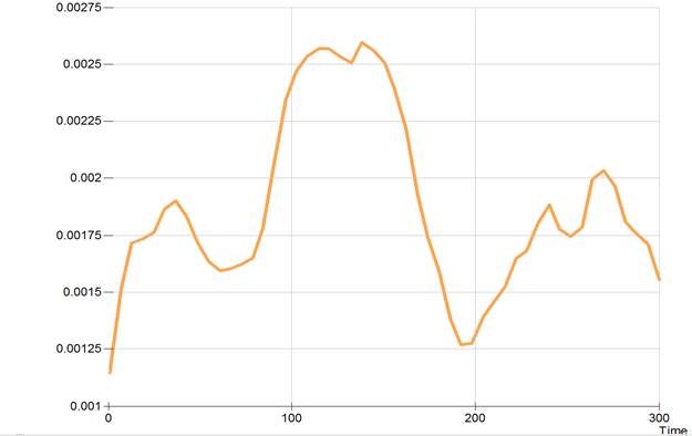
Adding the TABLE option to the SMOOTH command prints a table of the smoothed hazard estimates over the sepcified range. By default, the hazard is evaluated at 50 equally spaced points on this range. Howewver, the POINTS option can be used to change the number of points. The table gives the estimated hazard along with an estimate of the standard error of this estimate and upper and lower confidence bounds for the hazard. The default is for 95% confidence bounds unless this has been changed using the FITOPT CI command. The command

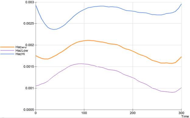
SMOOTH 100 CI TABLE TLIM 0 300 @

requests a smoothed hazard function plot with pointwise confidence bounds over the range of 0 to 300 days with a smoothng bandwidth of 100 days with the smoothed hazard data written to the log file.

The smoothed hazard table is given below:

Smoothed hazard summary table

Multiplicative 95% Confidence bounds

Time Hazard Std. Err. Lower Upper

--------- --------- ---------- --------- ---------

1.0000 0.001752 1.297 0.001053 0.002915

6.9800 0.001713 1.271 0.001070 0.002741

12.960 0.001691 1.247 0.001097 0.002605

18.940 0.001673 1.226 0.001122 0.002493

24.920 0.001676 1.205 0.001162 0.002417

30.900 0.001700 1.186 0.001216 0.002377

36.880 0.001733 1.171 0.001271 0.002362

42.860 0.001768 1.161 0.001321 0.002368

48.840 0.001808 1.154 0.001366 0.002392

54.820 0.001849 1.150 0.001407 0.002431

60.800 0.001894 1.148 0.001445 0.002480

66.780 0.001944 1.147 0.001486 0.002543

72.760 0.001992 1.147 0.001521 0.002608

78.740 0.002030 1.150 0.001545 0.002669

84.720 0.002061 1.153 0.001559 0.002723

90.700 0.002084 1.156 0.001568 0.002772

96.680 0.002096 1.161 0.001565 0.002808

102.66 0.002103 1.165 0.001559 0.002838

108.64 0.002110 1.169 0.001553 0.002866

114.62 0.002105 1.174 0.001537 0.002882

120.60 0.002098 1.178 0.001521 0.002893

126.58 0.002086 1.183 0.001501 0.002897

132.56 0.002078 1.186 0.001487 0.002902

138.54 0.002071 1.189 0.001476 0.002907

144.52 0.002054 1.192 0.001455 0.002900

150.50 0.002033 1.196 0.001431 0.002889

156.48 0.002027 1.198 0.001421 0.002890

162.46 0.002019 1.201 0.001411 0.002888

168.44 0.002006 1.203 0.001396 0.002883

174.42 0.001976 1.208 0.001365 0.002860

180.40 0.001936 1.213 0.001326 0.002828

186.38 0.001908 1.218 0.001297 0.002807

192.36 0.001893 1.221 0.001279 0.002801

198.34 0.001869 1.227 0.001251 0.002791

204.32 0.001840 1.234 0.001218 0.002780

210.30 0.001801 1.243 0.001175 0.002761

216.28 0.001771 1.252 0.001141 0.002750

222.26 0.001752 1.259 0.001116 0.002750

228.24 0.001725 1.267 0.001085 0.002744

234.22 0.001688 1.278 0.001044 0.002728

240.20 0.001644 1.289 0.0009993 0.002706

246.18 0.001627 1.296 0.0009781 0.002706

252.16 0.001602 1.305 0.0009499 0.002700

258.14 0.001582 1.313 0.0009269 0.002699

264.12 0.001580 1.318 0.0009201 0.002714

270.10 0.001584 1.321 0.0009183 0.002733

276.08 0.001572 1.327 0.0009030 0.002738

282.06 0.001573 1.330 0.0008993 0.002750

288.04 0.001591 1.329 0.0009109 0.002779

294.02 0.001654 1.321 0.0009594 0.002853

300.00 0.001729 1.315 0.001011 0.002957

The hazard function plot is as follows.