Case-Cohort Data

The likelihood equations for case-cohort data were taken from the original paper by Prentice (1986) in which he proposed the case-cohort design. From a cohort of size , a subcohort of size is obtained by simple random sampling.

The quantities , , and are as defined above. As given by Prentice, the estimates of the relative risk are obtained from the pseudo-likelihood, namely,

(A.4)

where is now the set of all members of the risk set who are also in the subcohort sample and the case at . differs from , which was a set of all members of the risk set.

The likelihood is the product over all subjects in the cohort; factors in expression 8.4 may differ from one only for cases and members of . This implies that, although only the covariate vector for cases and the subcohort are directly used in parameter estimation, the full cohort must be followed to determine and, in particular, .

The maximum pseudo-likelihood estimate, , for is the quantity that nullifies the partial derivatives of the logarithm pseudo-likelihood, namely,

(8.5)

where

Using a Taylor's series expansion, a consistent estimate of the covariance matrix for is given by the so-called “sandwich” estimator , where is the matrix of mixed partial derivatives of the log likelihood and is the covariance matrix of at .

In place of the matrix of mixed partial derivatives, PEANUTS uses the more easily computed quantity obtained from expression 3 with replacing .

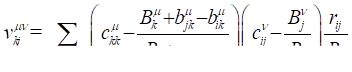
The covariance matrix of requires extensive calculations because of . The element of is given by

(A.6)

Since the pseudo-likelihood conditions on noncensored failure times, we have for all censored failure times, that is, with .

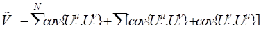
For each noncensored failure time, with , the element of the covariance matrix of is given by the usual expectation of , namely,

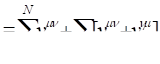
where

and

Next, let be an indicator function that takes value 1 if the failure at time occurs outside the subcohort and value 0 otherwise. Suppose with the case occurring within the subcohort, . Then , since is fixed, because the risk set at , , consists only of subcohort members and, conditional on all covariate and censoring histories up to , can be fully characterized. With =1, conditioning on covariate and censoring histories and the observed exposures at , we cannot know for certain which of the members is the case and therefore not in the subcohort, and thus we cannot know the composition of . This randomness induces the covariance between and . Prentice specifies the covariance as

A similar expression is obtained for . Note that because of differences in the composition of and and possible covariate changes over time, may not equal .

Expression 7 can then be rewritten as

In the case of ties in the failure times of noncensored cases, Prentice suggests modifying the likelihood using the methods given by Peto (1972) and Breslow (1974) for the partial likelihood, namely,

where is the number of ties.

The subcohort is selected at the start of follow-up. One possible disadvantage of the case-cohort approach occurs when there is substantial censoring; there may be no members of the subcohort to compare with later-occurring cases. Prentice (1986) and others have suggested that this problem can be minimized by sampling one or more additional subcohorts. Because the covariance between scores depends on the sampling, the equations provided above are not valid for all types of repeated subcohort sampling schemes. However, the formulae are valid for the important special cases where the subsequent subcohort is a simple random sample from the remaining cohort; in particular, the formulae are valid when a subsequent subcohort includes all remaining cohort members. Members of a new sample are “entered” through the use of a late entry (or left-truncation) variable with the EPICURE command ENTRY varname @. The estimated baseline survival curve (see below) is valid only if the sampling fraction is the same for all subcohort selections.

SCURVCSCHRT fraction @ command.

SCURV